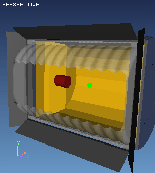
"Filled" representation of Optical System
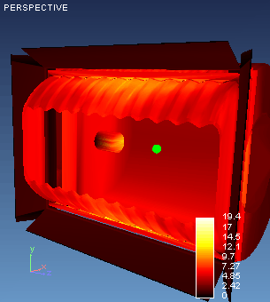
"Surface Map" representation of Optical System
Surface Maps allow you to check and analyze distribution of some surface characteristics over each surface of Elements included into your Project.
Currently used scale is shown at the bottom left corner of 3D Viewer.
In order to choose “Surface map” command (if it is not ordered yet) one should first, call contextual menu by right mouse button, put mouse marker onto corresponding row and press left button. The fact of regime ordering is marked in menu by bullet in the “Surface map” row. (See picture above). Regime may be cancelled by repeated pressing of left mouse button when marker is placed onto the same row. The ordering of “Filled” command cancels “Surface map” regime forcedly.
Example of “Filled” / “Surface map” switching:
|
|
|
|
"Filled" representation of Optical System |
"Surface Map" representation of Optical System |
All other Viewer options (image rotating and scaling, changing projections, adding/hiding layout components) can be used in various combinations both for “Surface map” and other regimes.
The table at the “Surface map” field contains absolute values in lk.
Filled – command, which, if ordered, displays elements of optical system as solid bodies.
It is reasonable to order “On” value of “Energy distribution” key only for those surfaces, which absorption is not zero.
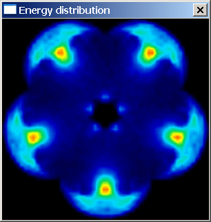
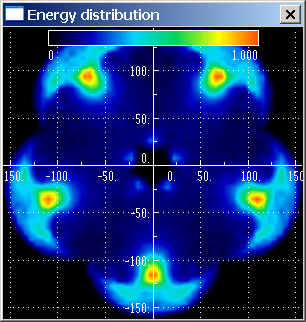
With Application, you are able to check spatial distribution of energy within you Optical System. To provide it, whole bounding box containing Optical System under analysis is divided by sections forming set of elementary cells. Number of section planes affecting accuracy of representation of spatial distribution of energy is set with Section parameter of Quality options of analysis. Energy distribution is considered as average spatial illuminosity within elementary cell.
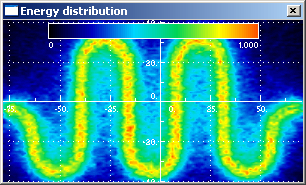
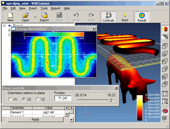
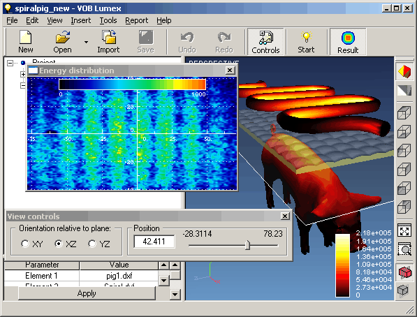
To check spatial distribution of energy Energy Distribution window is used. It contains a two-dimensional map of illuminosity distribution at chosen cross-section of bounding box containing your System with analysis plane. Typical view of Energy distribution is shown below:
You can open Energy distribution window anytime you want to check result of progress of analysis procedure dynamically.
You can check how duration of system analysis affect energy distributionaffecting of analysis duration spatial distribution of energy dynamically within bounding box of your System. To provide it .
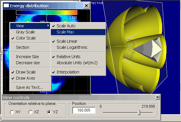
Analysis plane is parallel to cardinal planes of Global Coordinate System. Control of analysis plane is performed using View Controls window shown below:
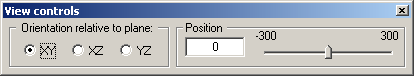
You can Work with View Controls window in the same manner as it described within Section View chapter. All changes will affect Energy distribution window immediately.
 |
 |
|
Analysis Plane position: Y=71.241 mm |
Analysis Plane position: Y=42.411 mm |
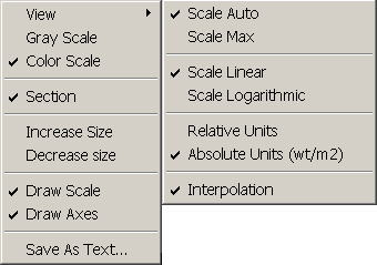
Energy distribution window provides some additional possibilities to evaluate analysis results that can be realized through context menu of window.
Context menu several triggered options dealing with visualization mode:
 |
|
Example of setting viewing parameters using context menu is shown below:
All changes may be applied during analysis procedure. Some examples of affecting different settings are shown below:
 |
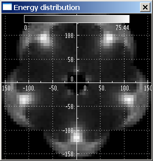 |
|
| Color scale, with interpolation | Gray scale, without interpolation | Color scale without axes and legend |
For more accurate analysis of energy distribution within currently chosen layer you can use cross-sections of map parallel to window sides. Cross-sections are visualized with two branch window placed as default at the bottom and right side from Energy distribution window as it shown below:
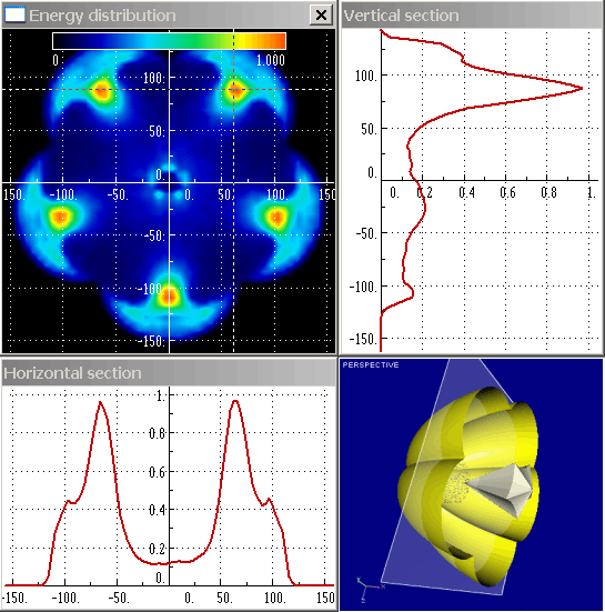
At the bottom left corner currently analyzed optical system is shown.
As a default, both cross-sections are passed through center of Energy distribution window and intersected, correspondingly, at the point with 0,0 coordinate. You can set any intersection point you want using your pointing device. For example, at the figure above intersection point is set at the (65,80) point. Places of sections are shown on energy distribution map with dashed lines.
You can also check energy distribution map dynamically moving intersection point with your pointing device.
You can change view of cross-section window and duplicate it using context menu shown below:
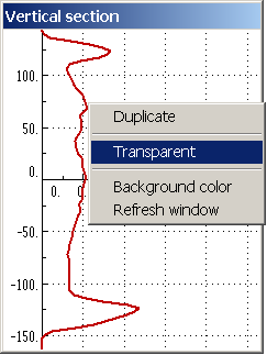 |
|
You can use copies of section window to compare energy distribution in different position or temporal changing of energy at the same position. To distinguish different sections you can use different background colors. With using transparent background of copied section window you can overlay several graph for easier comparison.
Note it is recommended to apply transparent background to copy of section window only.
Energy Indicatrix specifies angular distribution of radiation intensity emitted with Optical System. Energy indicatrix is calculated during general analysis routine and represented with polar diagram as it shown below:
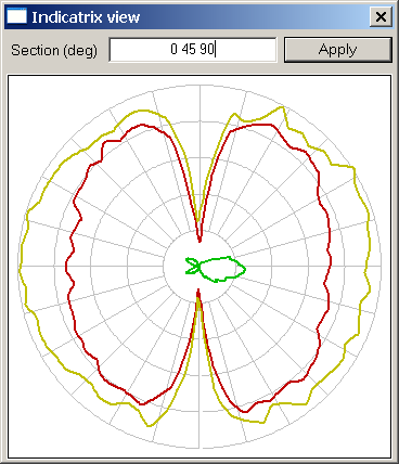
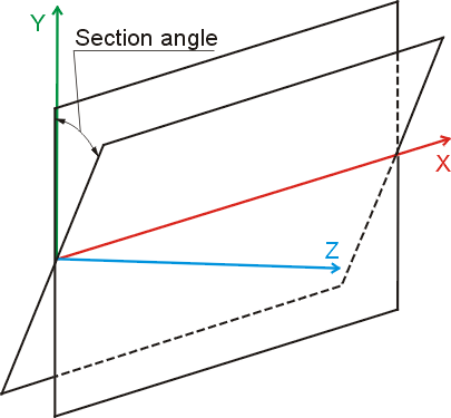
Polar diagram is based on all rays emitted out of Bounding Box of Optical System within any plane containing 0X axis as it shown on figure below. Section of interest is specified using section angle. Zero plane corresponds to X0Y section, positive angles are defined according to right-hand rule as it shown below:
You can visualize multiply view of energy indicatrix section on the same window. As a default, zero plane and 90 degree plane are visualized. There is textbox containing set of currently used sections at the top part of Indicatrix view window. Values of angles corresponding different sections are separated with white spaces. For example, on the figure shown above polar diagrams corresponding zero plane, 45 degree plane, and 90 degree plane are visualized.
You can add or remove polar diagram sections into Indicatrix view window anytime you want.
To set desired planes of energy indicatrix analysis: